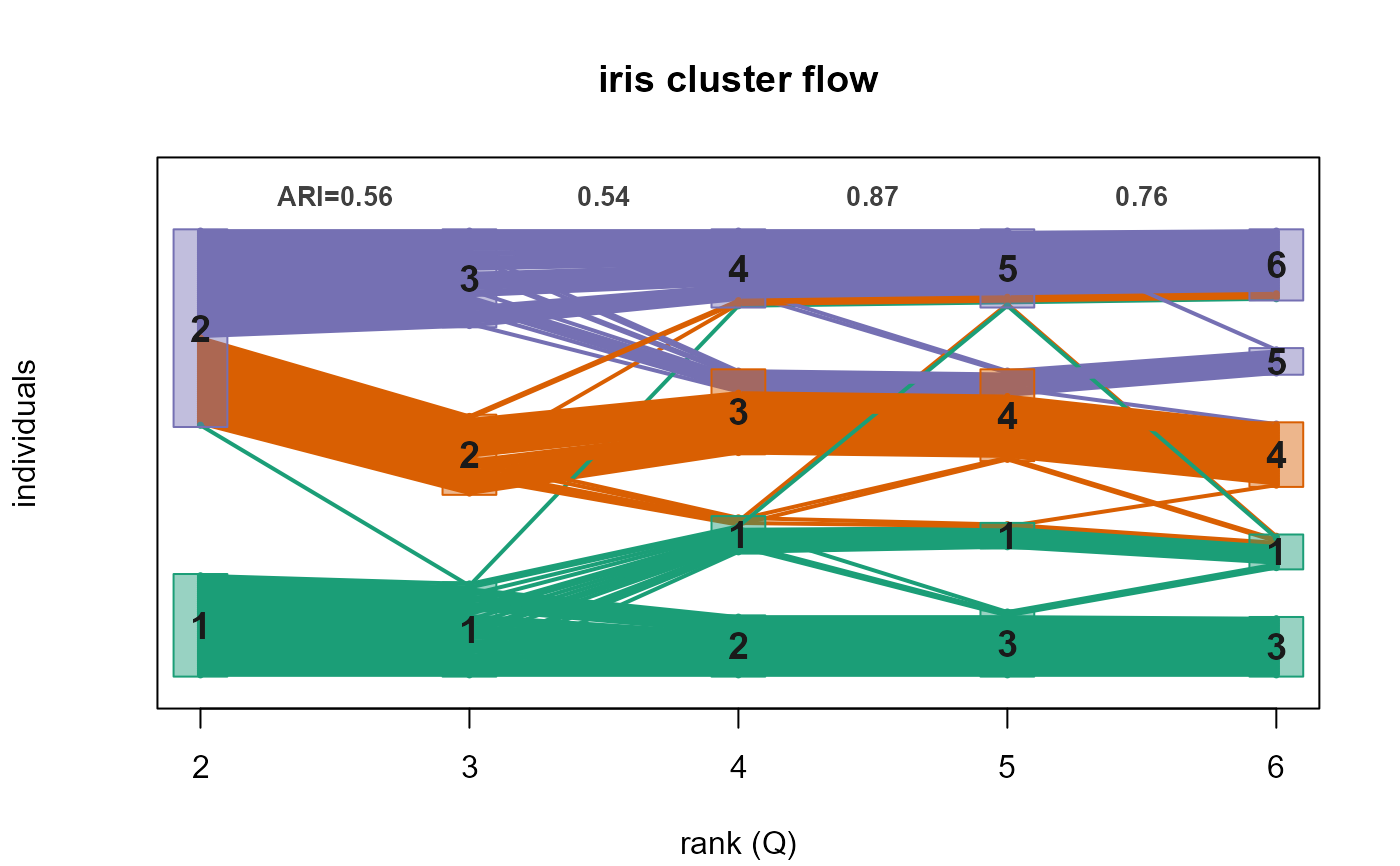
Visualizes how the hard sample clustering changes across a sequence of
fitted models – typically the same model at increasing ranks, but
also different models at the same rank. Each individual is a line
flowing left-to-right across the results (x-axis); its vertical
position at each result is determined by its cluster, and clusters are
reordered (barycenter method) to reduce crossings. Lines are coloured
by the individual's cluster in the reference result, so one can
see how the reference clusters split or merge. The adjusted Rand
index (ARI) between each pair of adjacent results is printed along the
top of the figure. X-axis ticks default to each result's $rank
and can be overridden with names.
Works for any non-negative multiplicative-update family
(nmfkc, nmfae, nmfkc.net, nmfre,
and the signed variants); the hard label is the argmax of the
coefficient/score matrix.
Arguments
- fits
A list (length \(\ge 2\)) of fitted models, all over the same \(N\) individuals. The results are taken in the given order (not sorted), so they may be different ranks or different models at the same rank.
- reference
The index (1-based position in
fits) of the result whose clustering defines the line colours. Defaults to the central result,floor(length(fits) / 2) + 1(e.g.\ the 2nd of 2 or 3 results).- names
Optional character vector (length
length(fits)) of x-axis tick labels. Defaults to each result's$rank.- plot
Logical; draw the diagram immediately by calling
plot.nmf.cluster.flow(defaultTRUE). SetFALSEto only build the object and plot it later.- ...
When
plot = TRUE, graphical arguments forwarded toplot.nmf.cluster.flow(e.g.\col,lwd,xlab,ylab,main).
Value
An object of class "nmf.cluster.flow" (returned
invisibly): a list with clusters (the \(N \times R\) table:
rows = individuals, columns = results, entries = cluster number = the
dominant-factor index of each fit, so it matches the factor/basis
numbering of fits; a factor that never dominates leaves an
empty, unused cluster number),
ypos (the layout positions), ranks (each result's
rank), labels (the x-axis labels), reference (the
reference index), ref.cluster (the reference hard labels),
ARI (adjusted Rand index between each pair of adjacent
results, length \(R - 1\)), and colors
(the default per-individual reference colour). Call
plot on it to (re)draw the diagram.
Examples
# \donttest{
Y <- t(as.matrix(iris[, 1:4]))
fits <- lapply(2:6, function(q) nmfkc(Y, Q = q, print.dims = FALSE))
fl <- nmf.cluster.flow(fits, reference = 2, plot = FALSE)  # 2nd result
head(fl$clusters)
#>    2 3 4 5 6
#> i1 1 1 2 3 3
#> i2 1 1 1 1 1
#> i3 1 1 2 3 3
#> i4 1 1 2 3 3
#> i5 1 1 2 3 3
#> i6 1 1 2 3 3
plot(fl, lwd = 2, main = "iris cluster flow")

# }
# }