NMF-RE: Mixed-Effects Modeling with nmfkc

Introduction

This vignette demonstrates NMF-RE (Non-negative Matrix Factorization with Random Effects), a mixed-effects extension of NMF implemented in the nmfkc package.

Why Mixed Effects?

Standard NMF with covariates models the data as: \[Y \approx X \Theta A\]

where \(\Theta A\) captures systematic (fixed) effects of covariates \(A\) on latent scores. However, in many applications — such as longitudinal studies, panel data, or clustered observations — individuals exhibit unit-specific deviations that cannot be explained by covariates alone.

NMF-RE addresses this by adding random effects \(U\): \[Y = X(\Theta A + U) + \mathcal{E}\]

• \(Y\) (\(P \times N\)): Non-negative observation matrix (e.g., repeated measurements over \(P\) time points for \(N\) subjects).
• \(X\) (\(P \times Q\)): Non-negative basis matrix learned from data.
• \(\Theta\) (\(Q \times K\)): Coefficient matrix for covariate effects.
• \(A\) (\(K \times N\)): Covariate matrix (e.g., intercept, sex, treatment).
• \(U\) (\(Q \times N\)): Random effects matrix capturing individual deviations.
• \(\mathcal{E}\): Residual noise with variance \(\sigma^2\).

The random effects \(U\) follow a ridge-type prior controlled by variance \(\tau^2\), and the penalty \(\lambda = \sigma^2 / \tau^2\) determines the degree of shrinkage.

Key Features

• Automatic regularization: df.rate controls the effective degrees of freedom consumed by \(U\), preventing overfitting.
• Wild bootstrap inference: Standard errors, z-values, p-values, and confidence intervals for \(\Theta\) without repeated constrained re-optimization.
• Trace-based ICC: Quantifies the proportion of variance attributable to random effects.

---

1. Data: Orthodont (Longitudinal Growth)

We use the Orthodont dataset from the nlme package: orthodontic distance measurements for 27 children at ages 8, 10, 12, and 14. The covariate of interest is sex (Male/Female).

library(nmfkc)
library(nlme)
#> Warning: package 'nlme' was built under R version 4.4.3

data(Orthodont)
head(Orthodont)
#> Grouped Data: distance ~ age | Subject
#>   distance age Subject  Sex
#> 1     26.0   8     M01 Male
#> 2     25.0  10     M01 Male
#> 3     29.0  12     M01 Male
#> 4     31.0  14     M01 Male
#> 5     21.5   8     M02 Male
#> 6     22.5  10     M02 Male

1.1 Prepare the Observation Matrix Y

Each column of \(Y\) is a subject, each row is a time point (age). Since there are 4 ages and 27 subjects, \(Y\) is \(4 \times 27\).

Y <- matrix(Orthodont$distance, nrow = 4, ncol = 27)
colnames(Y) <- paste0("S", 1:27)
rownames(Y) <- paste("Age", c(8, 10, 12, 14))
Y[, 1:6]
#>        S1   S2   S3   S4   S5   S6
#> Age 8  26 21.5 23.0 25.5 20.0 24.5
#> Age 10 25 22.5 22.5 27.5 23.5 25.5
#> Age 12 29 23.0 24.0 26.5 22.5 27.0
#> Age 14 31 26.5 27.5 27.0 26.0 28.5

1.2 Prepare the Covariate Matrix A

We create a \(2 \times 27\) covariate matrix with an intercept row and a binary male indicator.

male <- ifelse(Orthodont$Sex[seq(1, 108, 4)] == "Male", 1, 0)
A <- rbind(intercept = 1, male = male)
A[, 1:6]
#>           [,1] [,2] [,3] [,4] [,5] [,6]
#> intercept    1    1    1    1    1    1
#> male         1    1    1    1    1    1

---

2. Selecting dfU Cap Rate

Before fitting the model, we use nmfre.dfU.scan() to scan different regularization levels. The dfU cap rate limits how many effective degrees of freedom the random effects \(U\) can consume, preventing overfitting.

The scan evaluates rates from 0.1 to 1.0 (where 1.0 means no cap). Key columns in the output:

• dfU: Effective degrees of freedom actually used.
• safeguard: Whether dfU stayed below the cap (TRUE = safe).
• hit: Whether \(\tau^2\) was updated freely (TRUE = unconstrained).
• ICC: Trace-based Intraclass Correlation Coefficient.

scan_result <- nmfre.dfU.scan(1:10/10, Y, A, rank = 1)
scan_result
#>    rate dfU.cap  dfU safeguard   hit converged  tau2 sigma2    ICC
#> 1   0.1     2.7 2.70     FALSE  TRUE      TRUE 0.443      1 0.0270
#> 2   0.2     5.4 5.40     FALSE  TRUE      TRUE 0.996      1 0.0588
#> 3   0.3     8.1 5.42      TRUE FALSE      TRUE 1.000      1 0.0590
#> 4   0.4    10.8 5.42      TRUE FALSE      TRUE 1.000      1 0.0590
#> 5   0.5    13.5 5.42      TRUE FALSE      TRUE 1.000      1 0.0590
#> 6   0.6    16.2 5.42      TRUE FALSE      TRUE 1.000      1 0.0590
#> 7   0.7    18.9 5.42      TRUE FALSE      TRUE 1.000      1 0.0590
#> 8   0.8    21.6 5.42      TRUE FALSE      TRUE 1.000      1 0.0590
#> 9   0.9    24.3 5.42      TRUE FALSE      TRUE 1.000      1 0.0590
#> 10  1.0    27.0 5.42      TRUE FALSE      TRUE 1.000      1 0.0590

Interpreting the Scan

A good df.rate satisfies two criteria:

1. safeguard = TRUE: The cap is not overly binding.
2. hit = TRUE: The model converges to a natural solution without the cap forcing an artificial penalty.

Choose the smallest rate where both conditions hold. This balances model flexibility against overfitting.

---

3. Fitting the NMF-RE Model

Based on the scan, we select df.rate = 0.2 and fit the model with rank = 1 (a single latent trend). The prefix argument labels the basis.

res <- nmfre(Y, A, rank = 1, df.rate = 0.2, prefix = "Trend")

3.1 Model Summary

summary() displays variance components, fit statistics, and the coefficient table with significance stars.

summary(res)
#> NMF-RE: Y(4,27) = X(4,1) [C(1,2) A + U(1,27)]
#> Iterations: 2 (converged, epsilon = 1e-05)
#> R-squared: 0.5654 (XB+blup), 0.4167 (XB)
#> 
#> Variance components:
#>   sigma2 = 1  (residual)
#>   tau2   = 0.9961  (random effect)
#>   lambda = 1.004  (sigma2 / tau2)
#>   ICC    = 0.0588  (tau2*tr(X'X) / (tau2*tr(X'X) + sigma2*P))
#>   dfU    = 5.40 <= 5.40 (cap rate = 0.20)
#> 
#> Coefficients:
#>                   Estimate Std. Error (Boot) z value   Pr(>z) 
#> intercept:Trend1    90.393      2.471  2.452   36.58   <2e-16 ***
#>      male:Trend1     9.606      3.056  2.977    3.14 0.0008356 ***
#> ---
#> Signif. codes:  0 '***' 0.001 '**' 0.01 '*' 0.05 '.' 0.1 ' ' 1

Understanding the Output

Variance components:

• \(\sigma^2\): Residual variance (measurement noise).
• \(\tau^2\): Random effect variance (individual heterogeneity).
• ICC: Proportion of variance from random effects. Higher ICC means stronger individual differences relative to noise.

Coefficient table (\(\Theta\)):

• Estimate: Effect of each covariate on the latent trend.
• Std. Error: From wild bootstrap.
• Pr(>|z|): One-sided p-value (H0: \(\Theta_{qk} = 0\) vs H1: \(\Theta_{qk} > 0\)), appropriate because \(\Theta\) is non-negative.

R-squared:

• \(R^2\) (XB+blup): Fit including both fixed and random effects.
• \(R^2\) (XB): Fit from fixed effects only — the gap shows how much random effects improve the fit.

---

4. Visualization

We plot the growth curves to see how the model captures both population-level trends (fixed effects) and individual deviations (random effects).

age <- c(8, 10, 12, 14)

plot(age, res$XB[, 1], type = "n", ylim = range(Y),
     xlab = "Age (years)", ylab = "Distance (mm)",
     main = "Orthodont: NMF-RE Growth Curves")

# Plot observed data points
for (j in 1:27) {
  pch_j <- ifelse(male[j] == 1, 4, 1)
  points(age, Y[, j], pch = pch_j, col = "gray60")
}

# Plot individual predictions (fixed + random effects)
for (j in 1:27) {
  lines(age, res$XB.blup[, j], col = "steelblue", lty = 3, lwd = 0.8)
}

# Plot population-level fixed effects (two lines: male and female)
for (j in 1:27) {
  lines(age, res$XB[, j], col = "red", lwd = 2)
}

legend("topleft",
  legend = c("Fixed effect (male/female)", "Fixed + Random (BLUP)",
             "Male (observed)", "Female (observed)"),
  lwd = c(2, 1, NA, NA), lty = c(1, 3, NA, NA),
  pch = c(NA, NA, 4, 1),
  col = c("red", "steelblue", "gray60", "gray60"),
  cex = 0.85)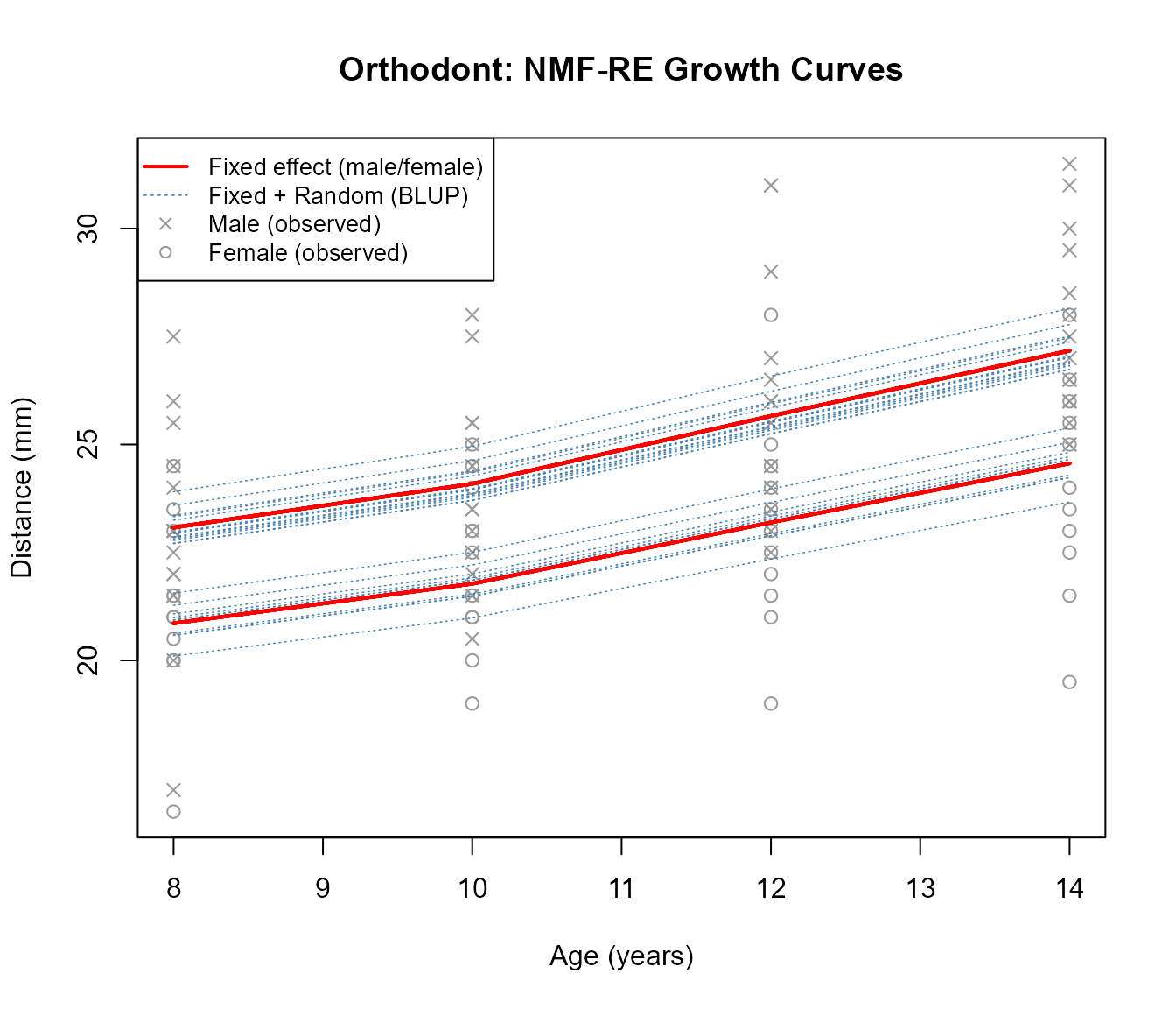

Interpreting the Plot

• Red solid lines: Population-level fitted values from fixed effects (\(X \Theta A\)). There are two distinct curves — one for males (higher) and one for females (lower) — reflecting the sex effect in \(\Theta\).
• Blue dashed lines: Individual-level predictions (\(X(\Theta A + U)\)). Each line is shifted from the population curve by the subject’s random effect \(U\), capturing personal growth trajectories.
• Gray points: Observed measurements. Crosses (\(\times\)) for males, circles (\(\circ\)) for females.

---

5. Examining Learned Components

5.1 Basis Matrix X

The basis \(X\) represents the latent temporal pattern shared across all subjects.

cat("Basis X (temporal pattern):\n")
#> Basis X (temporal pattern):
print(round(res$X, 4))
#>        Trend1
#> Age 8  0.2308
#> Age 10 0.2409
#> Age 12 0.2566
#> Age 14 0.2717

Since rank = 1, there is one basis vector. Its shape shows how the latent factor manifests across the four ages. The column is normalized to sum to 1.

5.2 Coefficient Matrix \(\Theta\)

\(\Theta\) maps covariates to latent scores:

cat("Coefficient matrix (Theta):\n")
#> Coefficient matrix (Theta):
print(round(res$C, 4))
#>        intercept   male
#> Trend1   90.3934 9.6059

• intercept: Baseline level of the latent trend for females.
• male: Additional contribution for males. A significant positive value indicates that males have higher orthodontic distances on average.

5.3 Random Effects U

\(U\) captures individual deviations. Subjects with positive \(U\) values grow faster than the population average; negative values indicate slower growth.

barplot(res$U[1, ], names.arg = colnames(Y),
        las = 2, cex.names = 0.7,
        col = ifelse(male == 1, "steelblue", "salmon"),
        main = "Random Effects (U) by Subject",
        ylab = "Random effect value")
legend("topright", fill = c("steelblue", "salmon"),
       legend = c("Male", "Female"), cex = 0.85)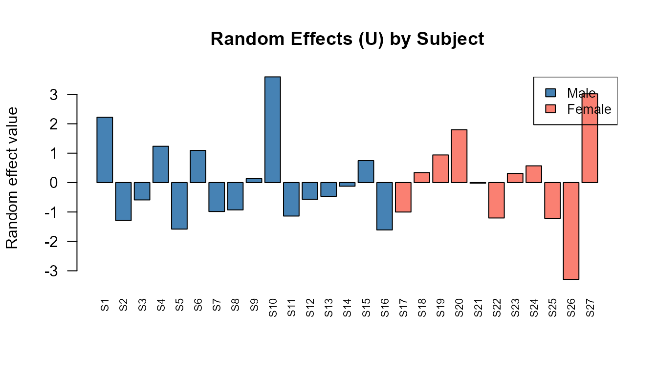

---

6. Model Diagnostics

6.1 Convergence

Check that the algorithm converged properly:

cat("Converged:", res$converged, "\n")
#> Converged: TRUE
cat("Iterations:", res$iter, "\n")
#> Iterations: 2
cat("Stop reason:", res$stop.reason, "\n")
#> Stop reason: epsilon

plot(res$objfunc.iter, type = "l",
     xlab = "Iteration", ylab = "Objective function",
     main = "Convergence Trace")

6.2 Residual Analysis

Compare the fitted values against the original data:

residuals <- Y - res$XB.blup
cat("Mean absolute residual (BLUP):", round(mean(abs(residuals)), 4), "\n")
#> Mean absolute residual (BLUP): 1.5118
cat("Mean absolute residual (fixed):", round(mean(abs(Y - res$XB)), 4), "\n")
#> Mean absolute residual (fixed): 1.7612

# Fitted vs Observed
plot(as.vector(Y), as.vector(res$XB.blup),
     xlab = "Observed", ylab = "Fitted (BLUP)",
     main = "Observed vs Fitted", pch = 16, col = "steelblue")
abline(0, 1, col = "red", lwd = 2)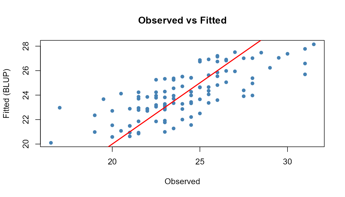

---

7. Comparison: With and Without Random Effects

To appreciate the value of random effects, compare NMF-RE with a standard NMF covariate model (no random effects).

# Standard NMF with covariates (no random effects)
res_fixed <- nmfkc(Y, A = A, rank = 1)
#> Y(4,27)~X(4,1)C(1,2)A(2,27)=XB(1,27)...0sec

cat("=== Standard NMF (fixed effects only) ===\n")
#> === Standard NMF (fixed effects only) ===
cat("R-squared:", round(1 - sum((Y - res_fixed$XB)^2) / sum((Y - mean(Y))^2), 4), "\n\n")
#> R-squared: 0.4161

cat("=== NMF-RE (fixed + random effects) ===\n")
#> === NMF-RE (fixed + random effects) ===
cat("R-squared (XB):      ", round(res$r.squared.fixed, 4), "\n")
#> R-squared (XB):       0.4167
cat("R-squared (XB+blup): ", round(res$r.squared, 4), "\n")
#> R-squared (XB+blup):  0.5654
cat("ICC:                 ", round(res$ICC, 4), "\n")
#> ICC:                  0.0588

The improvement from fixed-only \(R^2\) to BLUP \(R^2\) quantifies the contribution of individual random effects.

---

Separated Inference with nmfre.inference()

When fitting NMF-RE, you can separate optimization from statistical inference. First fit with wild.bootstrap = FALSE (faster), then run inference separately:

# Fit without bootstrap (fast)
res_fast <- nmfre(Y, A, rank = 1, df.rate = 0.2, prefix = "Trend",
                  wild.bootstrap = FALSE)

# Run inference separately
res_inf <- nmfre.inference(res_fast, Y, A, wild.B = 500)
res_inf$coefficients[, c("Basis", "Covariate", "Estimate", "SE", "p_value")]
#>    Basis Covariate  Estimate       SE       p_value
#> 1 Trend1 intercept 90.393445 2.471312 3.306544e-293
#> 2 Trend1      male  9.605879 3.056105  8.356231e-04

Visualization with nmfkc.DOT()

The inference result is compatible with nmfkc.DOT() for graph visualization. Edges are filtered by significance level and decorated with stars:

dot <- nmfkc.DOT(res_inf, type = "YXA", sig.level = 0.05)
plot(dot)

---

Summary

NMF-RE provides a principled way to model individual heterogeneity in NMF:

Step	Function	Purpose
1	nmfre.dfU.scan()	Select regularization level
2	nmfre()	Fit the mixed-effects model
3	summary()	Examine variance components and inference
4	nmfre.inference()	Separated inference (optional)
5	nmfkc.DOT()	Visualize with significance stars

When to use NMF-RE:

• Longitudinal or repeated-measures data where subjects differ systematically.
• Panel data with unit-level heterogeneity.
• Any NMF application where fixed covariates alone leave structured residual variation.

For more details on the underlying methodology, see:

• Satoh, K. (2026). Wild Bootstrap Inference for Non-Negative Matrix Factorization with Random Effects. arXiv:2603.01468. https://arxiv.org/abs/2603.01468