Topic Modeling with nmfkc
Source:vignettes/topic-modeling-with-nmfkc.Rmd
topic-modeling-with-nmfkc.RmdIntroduction
Non-negative Matrix Factorization (NMF) is a powerful technique for topic modeling. By decomposing a document-term matrix, we can simultaneously discover latent Topics (clusters of words) and their Trends (proportions in documents).
This vignette demonstrates how to use the nmfkc package
to analyze the U.S. presidential inaugural addresses using the
quanteda package.
We will cover:
-
Data Preparation: Converting text data into a
matrix format suitable for
nmfkc. - Rank Selection: Determining the optimal number of topics using robust Cross-Validation.
- Standard NMF: Extracting basic topics and interpreting key words.
- Kernel NMF: Modeling the temporal evolution of topics using the “Year” as a covariate.
First, let’s load the necessary packages.
1. Data Preparation
We create a Document-Feature Matrix (DFM) where rows represent documents and columns represent words.
# Load the corpus from quanteda
corp <- corpus(data_corpus_inaugural)

# Preprocessing: tokenize, remove stopwords, and punctuation
tok <- tokens(corp, remove_punct = TRUE)
tok <- tokens_remove(tok, pattern = stopwords("en", source = "snowball"))

# Create DFM and filter
df <- dfm(tok)
df <- dfm_select(df, min_nchar = 3) # Remove short words (<= 2 chars)
df <- dfm_trim(df, min_termfreq = 100) # Remove rare words (appearing < 100 times)

# --- CRITICAL STEP ---
# quanteda's DFM is (Documents x Words).
# nmfkc expects (Words x Documents).
# We must transpose the matrix.
d <- as.matrix(df)
# Sort by frequency
index <- order(colSums(d), decreasing=TRUE)
d <- d[,index]
Y <- t(d)

dim(Y) # Features (Words) x Samples (Documents)
#> [1] 67 59
2. Rank Selection (Number of Topics)
Before fitting the model, we need to decide the number of topics
(\(rank\)). The
nmfkc.rank() function helps us choose an appropriate
rank.
The default detail = "full" performs
Element-wise Cross-Validation (Wold’s CV). This method
randomly holds out individual matrix elements and evaluates how well the
model predicts them, providing a robust measure for rank selection
(though it takes more computation time).
# Evaluate ranks from 2 to 6
nmfkc.rank(Y, rank = 2:6)
#> Y(67,59)~X(67,2)B(2,59)...0sec
#> Y(67,59)~X(67,3)B(3,59)...0sec
#> Y(67,59)~X(67,4)B(4,59)...0sec
#> Y(67,59)~X(67,5)B(5,59)...0sec
#> Y(67,59)~X(67,6)B(6,59)...0sec
#> Running Element-wise CV (this may take time)...
#> Performing Element-wise CV for Q = 2,3,4,5,6 (5-fold)...
#> Note: sample-clustering quality (silhouette / CPCC / dist.cor) is not part of rank selection; compute it from a list of fits with nmf.cluster.criteria(). See ?nmf.cluster.criteria![]()
Looking at the diagnostics (the minimum ECV Sigma and the elbow of
the R-squared curve; the green eff.rank line is shown for
context), let’s assume Rank = 3 is a reasonable choice
for this overview.
3. Standard NMF
We fit the standard NMF model (\(Y \approx
XB\)) with rank = 3. In the context of topic
modeling:
- \(X\) (Basis Matrix): Represents Topics (distribution of words).
- \(B\) (Coefficient Matrix): Represents Trends (distribution of topics across documents).
rank <- 3
# Set seed for reproducibility
res_std <- nmfkc(Y, rank = rank, seed = 123, prefix = "Topic")
#> Y(67,59)~X(67,3)B(3,59)...0sec

# Check Goodness of Fit (R-squared)
res_std$r.squared
#> [1] 0.6129089
Interpreting Topics (Keywords)
We can identify the meaning of each topic by looking at the words
with the highest weights in the basis matrix X.
# Extract top 10 words for each topic from X.prob (normalized X)
Xp <- res_std$X.prob
for(q in 1:rank){
  message(paste0("----- Featured words on Topic [", q, "] -----"))
  print(paste0(rownames(Xp), "(", rowSums(Y), ") ", round(100*Xp[,q], 1), "%")[Xp[,q]>=0.5])
}
#> ----- Featured words on Topic [1] -----
#>  [1] "government(564) 54.1%" "states(334) 62.7%"     "shall(316) 59.3%"
#>  [4] "public(225) 72%"       "united(203) 68.1%"     "union(190) 53.9%"
#>  [7] "war(181) 65.4%"        "national(158) 66.8%"   "congress(130) 60.1%"
#> [10] "laws(130) 81.2%"       "law(129) 60%"          "just(128) 56.9%"
#> [13] "interests(115) 57.6%"  "among(108) 62.9%"      "foreign(104) 72.2%"
#> ----- Featured words on Topic [2] -----
#>  [1] "may(343) 56.7%"          "one(267) 57.7%"
#>  [3] "power(241) 91%"          "constitution(209) 88.6%"
#>  [5] "spirit(140) 76.5%"       "rights(138) 62.4%"
#>  [7] "never(132) 57.2%"        "liberty(123) 69.8%"
#>  [9] "well(120) 61.2%"         "duty(120) 51%"
#> [11] "state(110) 76.1%"        "much(108) 53.3%"
#> [13] "powers(101) 65.7%"
#> ----- Featured words on Topic [3] -----
#>  [1] "must(376) 61.4%"     "world(319) 97.6%"    "nation(305) 63.6%"
#>  [4] "peace(258) 57.5%"    "new(250) 90.4%"      "time(220) 55.4%"
#>  [7] "america(202) 100%"   "nations(199) 57.8%"  "freedom(185) 80.3%"
#> [10] "american(172) 59.9%" "let(160) 99.8%"      "make(147) 56.1%"
#> [13] "justice(142) 52.1%"  "life(138) 73.9%"     "work(124) 90.9%"
#> [16] "hope(120) 64.3%"     "know(111) 100%"      "fellow(110) 57.3%"
#> [19] "history(105) 79.4%"  "today(105) 100%"
(Note: Interpretation depends on the result. For example, one topic might contain words like “government, people, states” (Political), while another might have “world, peace, freedom” (International).)
4. Kernel NMF: Temporal Topic Evolution
One of the unique features of nmfkc is Kernel
NMF. In standard NMF, the order of documents is ignored; each
speech is treated independently. However, inaugural addresses have a
strong temporal component. By using the “Year” as a
covariate, we can smooth the topic proportions over time to see
historical shifts.
Optimizing the Kernel Parameter
We construct a covariate matrix U using the year of the
address. We then find the optimal kernel bandwidth (beta)
using Cross-Validation.
# Covariate: Year of the address
years <- as.numeric(substring(names(data_corpus_inaugural), 1, 4))
U <- t(as.matrix(years))

# Optimize beta (Gaussian Kernel width)
# We test a specific range of betas to locate the minimum CV error.
beta_candidates <- c(0.2, 0.5, 1, 2, 5) / 10000

# Run CV to find the best beta
# Note: We use the same rank (rank=3) as selected above.
cv_res <- nmfkc.kernel.beta.cv(Y, rank = rank, U = U, beta = beta_candidates, plot = FALSE)
#> beta=2e-05...0.1sec
#> beta=5e-05...0sec
#> beta=1e-04...0.1sec
#> beta=2e-04...0sec
#> beta=5e-04...0sec
best_beta <- cv_res$beta
print(best_beta)
#> [1] 2e-04
Fitting Kernel NMF
Now we fit the model using the kernel matrix A. This
enforces that documents close in time (similar years) should have
similar topic distributions.
# Create Kernel Matrix
A <- nmfkc.kernel(U, beta = best_beta)

# Fit NMF with Kernel Covariates
res_ker <- nmfkc(Y, A = A, rank = rank, seed = 123, prefix = "Topic")
#> Y(67,59)~X(67,3)C(3,59)A(59,59)=XB(3,59)...0sec
Visualization: Standard vs Kernel NMF
Let’s compare how topic proportions change over time.
- Standard NMF (Top): Shows noisy fluctuations. It captures the specific content of each speech but misses the larger historical context.
- Kernel NMF (Bottom): Reveals smooth historical trends, showing how themes like “Nation Building” vs “Global Affairs” have evolved over centuries.
oldpar <- par(mfrow = c(2, 1), mar = c(4, 4, 2, 1))

# Prepare Axis Labels (Rounded to integers)
at_points <- seq(1, ncol(Y), length.out = 10)
labels_years <- round(seq(min(years), max(years), length.out = 10))

# 1. Standard NMF (Noisy)
barplot(res_std$B.prob, col = 2:(rank+1), border = NA, xaxt='n',
        main = "Standard NMF: Topic Proportions (Noisy)", ylab = "Probability")
axis(1, at = at_points, labels = labels_years)

# 2. Kernel NMF (Smooth trend)
barplot(res_ker$B.prob, col = 2:(rank+1), border = NA, xaxt='n',
        main = "Kernel NMF: Temporal Topic Evolution (Smooth)", ylab = "Probability")
axis(1, at = at_points, labels = labels_years)

# Legend
legend("topright", legend = paste("Topic", 1:rank), fill = 2:(rank+1), bg="white", cex=0.8)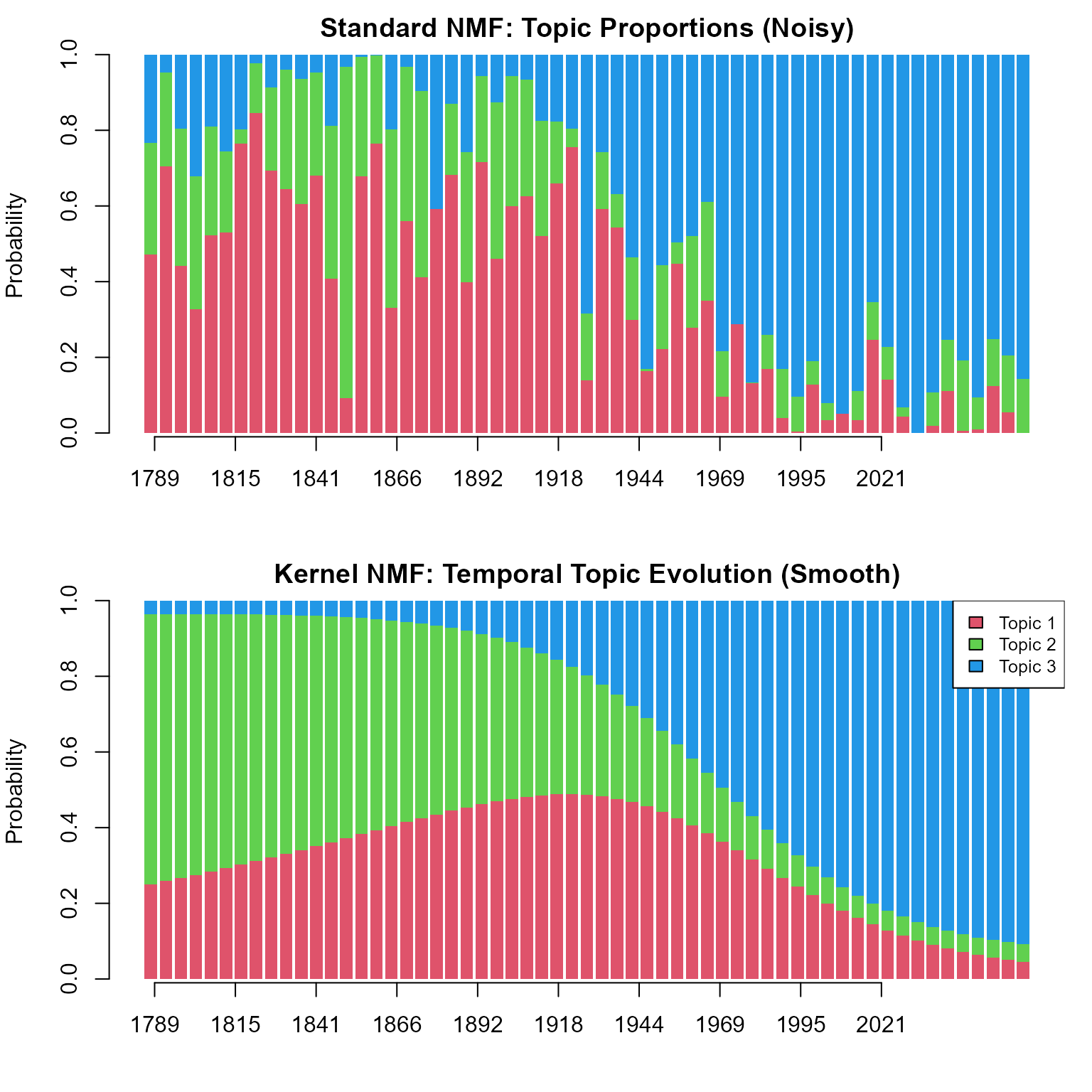
par(oldpar)