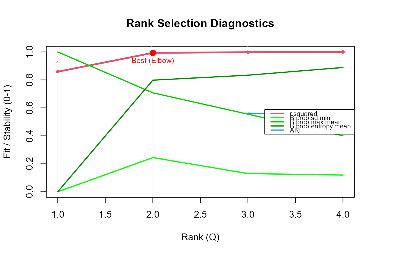
Rank selection diagnostics with graphical output

nmfkc.rank provides diagnostic criteria for selecting the rank (\(Q\)) in NMF with kernel covariates. Several model selection measures are computed (e.g., R-squared, silhouette, CPCC, ARI), and results can be visualized in a plot.

By default (save.time = FALSE), this function also computes the Element-wise Cross-Validation error (Wold's CV Sigma) using nmfkc.ecv.

The plot explicitly marks the "BEST" rank based on two criteria:

Elbow Method (Red): Based on the curvature of the R-squared values (always computed if Q > 2).
Min RMSE (Blue): Based on the minimum Element-wise CV Sigma (only if save.time=FALSE).

Usage

nmfkc.rank(Y, A = NULL, rank = 1:2, save.time = FALSE, plot = TRUE, ...)

Arguments

Y

Observation matrix.

A

Covariate matrix. If NULL, the identity matrix is used.

rank

A vector of candidate ranks to be evaluated.

save.time

Logical. If TRUE, skips heavy computations like Element-wise CV. Default is FALSE (computes everything).

plot

Logical. If TRUE (default), draws a plot of the diagnostic criteria.

...

Additional arguments passed to nmfkc and nmfkc.ecv.

Q: (Deprecated) Alias for rank.

Value

A list containing:

rank.best: The estimated optimal rank. Prioritizes ECV minimum if available, otherwise R-squared Elbow.
criteria: A data frame containing diagnostic metrics for each rank.

References

Brunet, J.P., Tamayo, P., Golub, T.R., Mesirov, J.P. (2004). Metagenes and molecular pattern discovery using matrix factorization. Proc. Natl. Acad. Sci. USA, 101, 4164–4169. doi:10.1073/pnas.0308531101 Punera, K., & Ghosh, J. (2008). Consensus-based ensembles of soft clusterings. Applied Artificial Intelligence, 22(7–8), 780–810. doi:10.1080/08839510802170546

Examples

# install.packages("remotes")
# remotes::install_github("ksatohds/nmfkc")
# Example.
library(nmfkc)
Y <- t(iris[,-5])
# Full run (default)
nmfkc.rank(Y, rank=1:4)
#> Y(4,150)~X(4,1)B(1,150)...
#> 0sec
#> Y(4,150)~X(4,2)B(2,150)...
#> 0sec
#> Y(4,150)~X(4,3)B(3,150)...
#> 0sec
#> Y(4,150)~X(4,4)B(4,150)...
#> 0sec
#> Running Element-wise CV (this may take time)...
#> Performing Element-wise CV for Q = 1,2,3,4 (5-fold)...
#> Y(4,150)~X(4,1)B(1,150)...
#> 0sec
#> Y(4,150)~X(4,1)B(1,150)...
#> 0sec
#> Y(4,150)~X(4,1)B(1,150)...
#> 0sec
#> Y(4,150)~X(4,1)B(1,150)...
#> 0sec
#> Y(4,150)~X(4,1)B(1,150)...
#> 0sec
#> Y(4,150)~X(4,2)B(2,150)...
#> 0sec
#> Y(4,150)~X(4,2)B(2,150)...
#> 0sec
#> Y(4,150)~X(4,2)B(2,150)...
#> 0sec
#> Y(4,150)~X(4,2)B(2,150)...
#> 0sec
#> Y(4,150)~X(4,2)B(2,150)...
#> 0sec
#> Y(4,150)~X(4,3)B(3,150)...
#> 0sec
#> Y(4,150)~X(4,3)B(3,150)...
#> 0sec
#> Y(4,150)~X(4,3)B(3,150)...
#> 0sec
#> Y(4,150)~X(4,3)B(3,150)...
#> 0sec
#> Y(4,150)~X(4,3)B(3,150)...
#> 0sec
#> Y(4,150)~X(4,4)B(4,150)...
#> 0sec
#> Y(4,150)~X(4,4)B(4,150)...
#> 0sec
#> Y(4,150)~X(4,4)B(4,150)...
#> 0sec
#> Y(4,150)~X(4,4)B(4,150)...
#> 0sec
#> Y(4,150)~X(4,4)B(4,150)...
#> 0sec

#> $rank.best
#> [1] 4
#> 
#> $criteria
#>   rank r.squared      ICp         AIC        BIC B.prob.sd.min       ARI
#> 1    1 0.8586795  52.4309   -50.91409   621.8162     0.0000000        NA
#> 2    2 0.9933479 102.3992 -1579.36199  -233.9015     0.2443194        NA
#> 3    3 0.9984511 153.9677 -2147.71982  -129.5291     0.1300233 0.5623250
#> 4    4 0.9999888 202.0625 -4800.29737 -2109.3764     0.1191841 0.5404919
#>   silhouette      CPCC  dist.cor sigma.ecv
#> 1         NA        NA 0.9410181 1.1694153
#> 2  0.8692814 0.9264254 0.9746472 0.7997277
#> 3  0.5358708 0.9193853 0.9489567 0.7786008
#> 4  0.3049893 0.8966046 0.9464434 0.7674663
#> 
# Fast run (skip ECV)
nmfkc.rank(Y, rank=1:4, save.time=TRUE)
#> Y(4,150)~X(4,1)B(1,150)...
#> 0sec
#> Y(4,150)~X(4,2)B(2,150)...
#> 0sec
#> Y(4,150)~X(4,3)B(3,150)...
#> 0sec
#> Y(4,150)~X(4,4)B(4,150)...
#> 0sec

#> $rank.best
#> [1] 2
#> 
#> $criteria
#>   rank r.squared      ICp         AIC        BIC B.prob.sd.min       ARI
#> 1    1 0.8586795  52.4309   -50.91409   621.8162     0.0000000        NA
#> 2    2 0.9933479 102.3992 -1579.36199  -233.9015     0.2443194        NA
#> 3    3 0.9984511 153.9677 -2147.71982  -129.5291     0.1300233 0.5623250
#> 4    4 0.9999888 202.0625 -4800.29737 -2109.3764     0.1191841 0.5404919
#>   silhouette CPCC dist.cor sigma.ecv
#> 1         NA   NA       NA        NA
#> 2         NA   NA       NA        NA
#> 3         NA   NA       NA        NA
#> 4         NA   NA       NA        NA
#>

References

Roy, O., & Vetterli, M. (2007). The effective rank: A measure of
effective dimensionality. Proc. 15th European Signal Processing
Conf. (EUSIPCO), 606–610. (effective.rank)
Wold, S. (1978). Cross-validatory estimation of the number of
components in factor and principal components models.
Technometrics, 20(4), 397–405.
doi:10.1080/00401706.1978.10489693
(sigma.ecv)
See also
nmfkc,
nmfkc.ecv (element-wise CV, used internally),
nmfkc.bicv (block bi-cross-validation),
nmfkc.consensus (stability) and
nmfkc.ard (Bayesian ARD) for alternative rank criteria.