Co-clustering two variable blocks with NMF-RRR (nmf.rrr) • nmfkc

Introduction

Many studies measure two blocks of variables on the same individuals – a block of covariates (inputs) and a block of responses (outputs) – and ask how groups of covariates relate to groups of responses. nmf.rrr() answers this by starting from the multivariate linear regression of the responses on the covariates and giving its non-negative regression coefficient matrix a tri-factorization

where (each column summing to one) softly clusters the response variables, (each row summing to one) softly clusters the covariate variables, and is a tested matrix of block correspondences. Because has rank , this is the non-negative, parts-based member of the reduced-rank regression (RRR) family – hence NMF-RRR – related to RRR as NMF is to PCA.

nmf.rrr() and its nmf.rrr.* helpers are the interface; the names emphasise the reduced-rank-regression reading. The former nmfae() family names were deprecated in 0.8.8 and removed in 0.9.8.

This vignette reproduces the Doubs example (community ecology), where a single dominant upstream–downstream gradient aligns both blocks, so the correspondence is a clean permutation.

library(nmfkc)

The Doubs data

The Doubs data (Verneaux, 1973) record 27 fish species and 11 environmental variables at 30 sites along a French river – a classic illustration of canonical (correspondence) analysis. We take the fish abundances as the response block and the environmental variables as the covariate block .

Each variable is mapped to by a per-variable min–max transform (nmfkc.normalize()), which makes the sign-free environmental variables non-negative, and both blocks are laid out as variables sites ().

data(doubs, package = "ade4")

# per-variable min-max to [0,1], then transpose to (variables x sites)
nz <- function(M) t(nmfkc.normalize(as.matrix(M)))
Y1 <- nz(doubs$fish)   # responses: 27 fish species x 30 sites
Y2 <- nz(doubs$env)    # covariates: 11 environment x 30 sites
dim(Y1)
#> [1] 27 30
dim(Y2)
#> [1] 11 30

Fitting NMF-RRR

Element-wise cross-validation (below) selects . Signed models and inference benefit from several k-means restarts, so we set nstart = 20 and a tight tolerance.

fit <- nmf.rrr(Y1, Y2, rank1 = 2, rank2 = 2,
               epsilon = 1e-8, nstart = 20, seed = 1)

# in-sample, column-centered R^2
Y1hat <- fit$X1 %*% fit$C %*% fit$X2 %*% Y2
R2 <- 1 - sum((Y1 - Y1hat)^2) / sum((Y1 - rowMeans(Y1))^2)
round(R2, 3)
#> [1] 0.435

The fit is R2 = 0.435, reproducing the classical longitudinal zonation of the river.

Response groups (fish guilds)

Each column of is a probability vector over the fish species; the top species per column name the guild.

for (q in 1:ncol(fit$X1))
  cat(sprintf("Resp%d: %s\n", q,
      paste(rownames(Y1)[order(-fit$X1[, q])[1:6]], collapse = ", ")))
#> Resp1: Neba, Phph, Satr, Cogo, Thth, Teso
#> Resp2: Alal, Ruru, Gogo, Acce, Baba, Titi

Resp1 is a cold-water upstream guild (brown trout Satr, Phph, Neba, Cogo, grayling Thth) and Resp2 a warm-water downstream guild (roach Ruru, Gogo, barbel Baba, Alal).

Covariate groups (environmental gradients)

Each row of is a probability vector over the environmental variables.

for (r in 1:nrow(fit$X2))
  cat(sprintf("Cov%d: %s\n", r,
      paste(rownames(Y2)[order(-fit$X2[r, ])[1:5]], collapse = ", ")))
#> Cov1: dfs, flo, har, nit, pH
#> Cov2: oxy, alt, pH, slo, har

Cov1 is a nutrient / downstream gradient (distance from source dfs, flow flo, nitrate nit, BOD bdo) and Cov2 an oxic / upstream gradient (dissolved oxygen oxy, altitude alt, pH, slope slo).

Choosing the two ranks

Because the attainable fit is bounded by , the in-sample fit cannot choose the ranks; we use element-wise cross-validation (nmf.rrr.ecv()), which holds out entries of and predicts them.

ecv <- nmf.rrr.ecv(Y1, Y2, rank1 = 1:2, rank2 = 1:2,
                   nfolds = 5, seed = 123)
#> Element-wise CV: 4 (Q,R) pairs, 5-fold, 20 tasks...
#>   Q=1, R=1: MSE=0.090948, sigma=0.3016
#>   Q=2, R=1: MSE=0.090948, sigma=0.3016
#>   Q=1, R=2: MSE=0.090954, sigma=0.3016
#>   Q=2, R=2: MSE=0.065768, sigma=0.2565
round(ecv$sigma, 4)
#> Q=1,R=1 Q=2,R=1 Q=1,R=2 Q=2,R=2 
#>  0.3016  0.3016  0.3016  0.2565

The smallest hold-out error is at .

Inference for the correspondence matrix

The entries of say how strongly each covariate group drives each response group. nmf.rrr.inference() attaches standard errors (Fisher + wild bootstrap) and a one-sided boundary test (each ).

inf <- nmf.rrr.inference(fit, Y1, Y2)
co  <- inf$coefficients
print(format(co[order(co$p_value), c("Basis","Covariate","Estimate","SE","z_value","p_value")],
             digits = 3))
#>   Basis Covariate Estimate    SE  z_value  p_value
#> 3 Resp1      Cov2 3.97e+00 0.505 7.86e+00 1.93e-15
#> 2 Resp2      Cov1 1.40e+01 1.837 7.65e+00 1.03e-14
#> 1 Resp1      Cov1 2.06e-48 0.603 3.42e-48 5.00e-01
#> 4 Resp2      Cov2 9.54e-27 1.004 9.51e-27 5.00e-01

is a near-permutation: the upstream guild is driven by the oxic gradient and the downstream guild by the nutrient gradient (both ), while the two off-diagonal paths are essentially zero ().

round(fit$C, 3)
#>         Cov1  Cov2
#> Resp1  0.000 3.971
#> Resp2 14.049 0.000

Visualising and the two co-clusterings

nmf.rrr.heatmap() shows the response basis , the correspondence , and the covariate basis together.

nmf.rrr.heatmap(fit)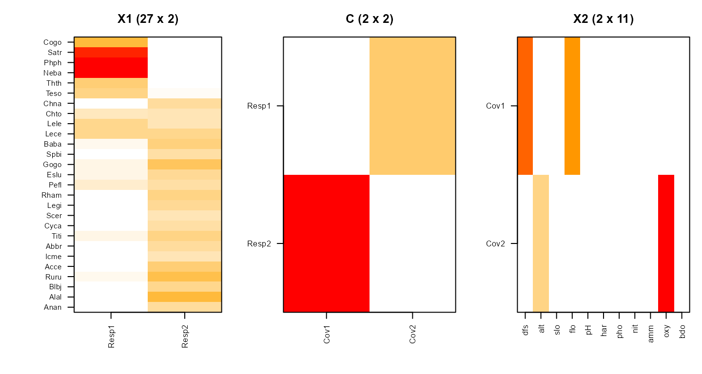

Clustering the individuals as well as the variables

The same fit clusters the sites. The two score matrices

give each site a profile over the covariate groups and over the response groups; column-normalising them yields soft memberships (B2.prob, B1.prob), and the arg-max gives hard labels (B2.cluster, B1.cluster). So a single model produces four groupings: two of variables (, ) and two of individuals (, ).

max(abs(fit$B1 - fit$C %*% fit$X2 %*% Y2))   # B1 = Theta B2, to machine precision
#> [1] 0

The Doubs sites are numbered from the source (1) downstream to (30), and that order is never given to the model. A labelling that comes out contiguous along the river is therefore a genuine recovery of the longitudinal gradient, not something the fit was told.

runs <- function(cl, tag) {
  cl <- as.vector(cl); r <- rle(cl)
  cat(sprintf("%-4s %s\n", tag, paste(cl, collapse = " ")))
  cat(sprintf("%-4s %d run(s): %s\n", "", length(r$lengths),
              paste(sprintf("%s x%d", r$values, r$lengths), collapse = " | ")))
  if (length(r$lengths) == 2)
    cat(sprintf("%-4s one break, between site %d and %d\n", "",
                r$lengths[1], r$lengths[1] + 1))
  cat("\n")
}
runs(fit$B1.cluster, "B1")   # response side: fish community
#> B1   1 1 1 1 1 1 1 1 1 1 2 2 2 2 2 2 2 2 2 2 2 2 2 2 2 2 2 2 2 2
#>      2 run(s): 1 x10 | 2 x20
#>      one break, between site 10 and 11
runs(fit$B2.cluster, "B2")   # covariate side: environment
#> B2   2 2 2 2 2 2 2 2 2 2 2 2 2 2 2 2 2 2 2 2 1 1 1 1 1 1 1 1 1 1
#>      2 run(s): 2 x20 | 1 x10
#>      one break, between site 20 and 21

Each side splits the river once, but not at the same place: the fish community changes at site 10|11, the environment at 20|21. Sites 11–20 are already downstream-type in their fauna while their measured environment is still upstream-type – the fish respond before the environmental variables recorded here cross over.

The soft memberships show how sharp each transition is.

round(fit$B1.prob[, 8:13], 2)    # response side, around the 10|11 break
#>          8    9   10   11   12   13
#> Resp1 0.66 0.53 0.52 0.45 0.46 0.45
#> Resp2 0.34 0.47 0.48 0.55 0.54 0.55
round(fit$B2.prob[, 18:23], 2)   # covariate side, around the 20|21 break
#>        18  19   20   21   22   23
#> Cov1 0.39 0.4 0.43 0.51 0.52 0.71
#> Cov2 0.61 0.6 0.57 0.49 0.48 0.29

Mapping the clusters onto the river

doubs$xy holds schematic map coordinates for the 30 sites, so the two labellings can be drawn on the river itself.

xy <- doubs$xy
panel <- function(cl, upstream.level, main, brk) {
  fill <- ifelse(as.vector(cl) == upstream.level, "white", "black")
  plot(xy, type = "n", asp = 1, xlab = "x (km)", ylab = "y (km)", main = main)
  lines(xy, col = "grey60", lwd = 2)                    # river course
  points(xy, pch = 21, bg = fill, col = "black", cex = 1.6)
  text(xy, labels = 1:30, pos = 3, offset = 0.4, cex = 0.55)
  mid <- (xy[brk, ] + xy[brk + 1, ]) / 2                # mark the break
  points(mid, pch = 4, cex = 2, lwd = 2.5)
}
op <- par(mfrow = c(1, 2), mar = c(4, 4, 3, 1))
panel(fit$B1.cluster, 1, "B1: fish community", 10)
panel(fit$B2.cluster, 2, "B2: environment", 20)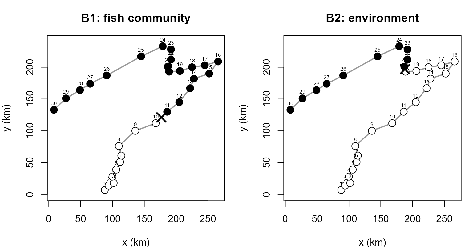

par(op)

Open circles are the upstream type, filled the downstream type, and the cross marks the break. Both transitions are single and contiguous, and the offset between them is the stretch where the two blocks disagree.

Whether supervision matters here is worth checking: k-means on either raw block, blind to the other block, is the natural baseline. Cluster labels are arbitrary, so agreement is measured in a label-switch-invariant way.

set.seed(1)
km1 <- kmeans(t(Y1), 2, nstart = 50)$cluster
km2 <- kmeans(t(Y2), 2, nstart = 50)$cluster
agree <- function(a, b) max(mean(a == b), mean(a != b))
c(B1.vs.kmY1 = agree(km1, as.vector(fit$B1.cluster)),
  B2.vs.kmY2 = agree(km2, as.vector(fit$B2.cluster)))
#> B1.vs.kmY1 B2.vs.kmY2 
#>  0.6000000  0.8666667
runs(km1, "km1")   # k-means on the fish block alone
#> km1  2 2 2 2 2 2 2 2 2 2 2 2 2 2 2 2 2 2 2 1 1 1 2 2 2 1 1 1 1 1
#>      4 run(s): 2 x19 | 1 x3 | 2 x3 | 1 x5
runs(km2, "km2")   # k-means on the environment block alone
#> km2  1 1 1 1 1 1 1 1 1 1 1 1 1 1 1 1 2 2 2 2 2 2 2 2 2 2 2 2 2 2
#>      2 run(s): 1 x16 | 2 x14
#>      one break, between site 16 and 17

The covariate side is close (0.87): the environmental gradient is strong enough that an unsupervised split of nearly reproduces . The response side is not (0.60). Left to itself, k-means on the fish block does not even return a contiguous stretch of river – it breaks late and then scatters a few sites back – because unsupervised clustering weights whatever variance dominates , gradient or not.

is contiguous because it is not computed from at all: it is , the environment read through the correspondence matrix. That is what supervision buys here, and it is also why the two site clusterings can be compared at all – they are tied to each other through , so the 10|11 versus 20|21 offset means something. The same model says which fish guild goes with which environmental gradient, and where along the river each one turns over.

Relation to other methods

Dropping non-negativity, at rank is ordinary reduced-rank regression (RRR): it attains a higher in-sample fit ( on Doubs) but returns signed loadings and no clusters. On these data the two share the dominant fitted direction (leading principal-angle cosine ); they differ in the basis of that subspace – non-negative parts versus signed singular directions – exactly as NMF relates to PCA. An unsupervised tri-NMF of the association recovers the same guilds and gradients here (the gradient is so dominant that supervised and unsupervised co-clusterings coincide), but, unlike NMF-RRR, cannot predict the community at a new site through .

When within-block and cross-block structure disagree – e.g. under – the non-negative, normalized parameterization of NMF-RRR stays well-behaved and exposes cross-structure (one response group driven by several covariate groups) that these baselines miss; see the paper for the nutrimouse and microbiome–metabolome examples.

References

Satoh, K. & Tokuda, Y. Co-clustering of Response and Covariate Variables by Tri-Factorizing Their Non-negative Regression Coefficient Matrix (manuscript).
Ding, C., Li, T., Peng, W. & Park, H. (2006). Orthogonal nonnegative matrix tri-factorizations for clustering. KDD.
Verneaux, J. (1973). Cours d’eau de Franche-Comté. PhD thesis. (Doubs data, R package ade4.) ```