Plot the latent dynamics of an NMF-VAR model

Draws the model's own dynamics — what the fit does — rather than the realized series. All of it lives in the \(Q\times Q\) latent transition matrices \(G_d=\Theta_d X\) returned by nmfkc.ar.latent, so every panel stays readable at a size the observed space cannot: a 47-region, 7-lag, rank-4 fit has \(47^2=2209\) observed impulse responses but only \(4^2=16\) latent ones.

Usage

# S3 method for class 'nmfkc.ar.latent'
plot(
  x,
  type = c("roots", "graph", "irf", "lag", "phase"),
  lag = NULL,
  horizon = 16L,
  ...
)

Arguments

x

An object from nmfkc.ar.latent.

type

Which panel to draw; see Details.

lag

Which lag to use for "graph" and "phase". Default NULL means \(\sum_d G_d\) for "graph" (the total one-step influence) and lag 1 for "phase".

horizon

Number of periods for "irf". Default 16.

...

Passed to the underlying plot call. "phase" also accepts start, a matrix of initial \(b_0\) values (one per row).

Value

invisible(NULL); called for the plot. "irf" and "lag" set up their own multi-panel layout and restore the previous one on exit.

Details

The available panels are

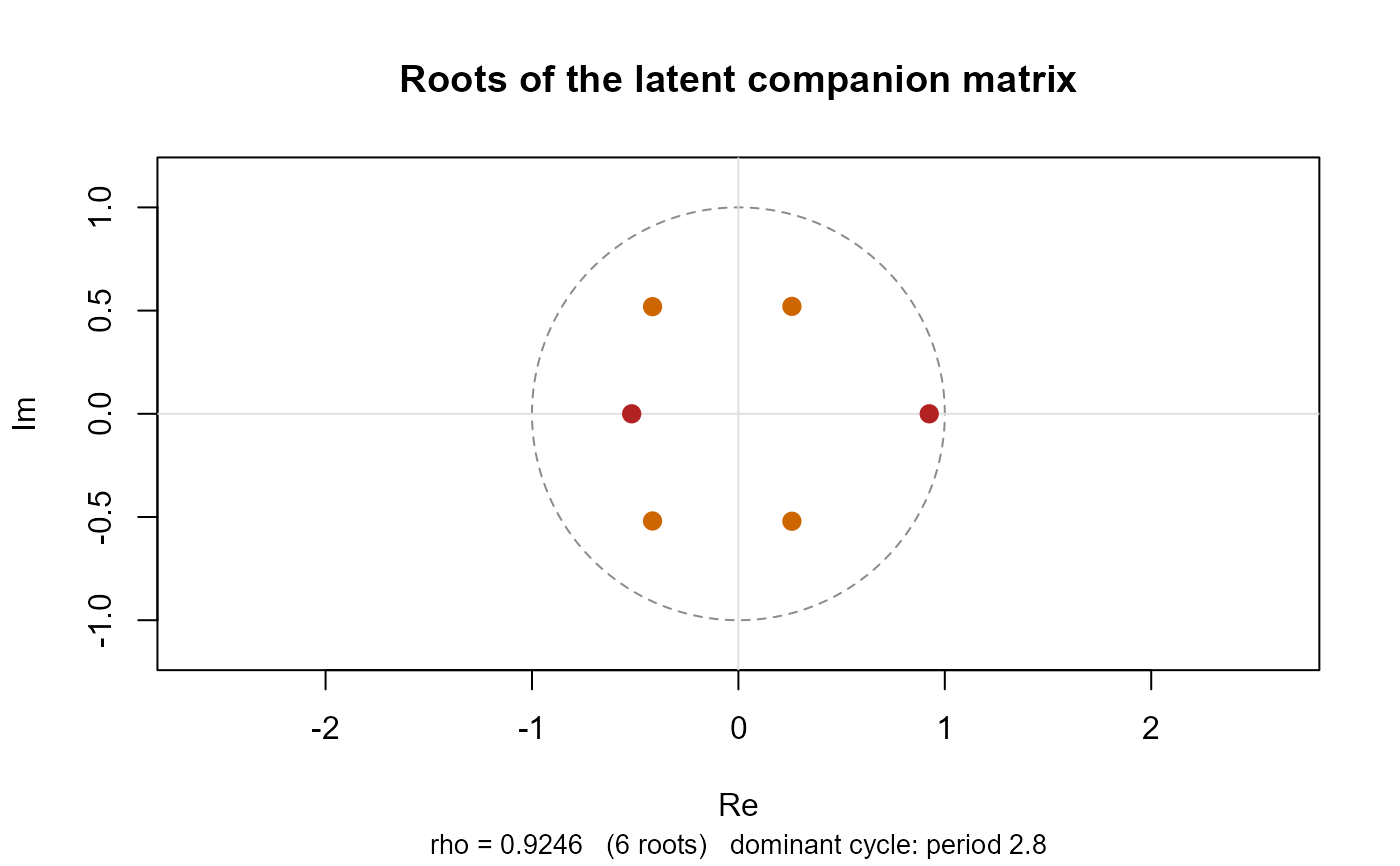
"roots"

(default) The \(DQ\) eigenvalues of the latent companion matrix on the unit circle. Complex roots are drawn in a different colour and their implied period is reported: a fit can sit near the boundary either because it cycles or because it is seasonal, and the spectral radius alone does not say which.

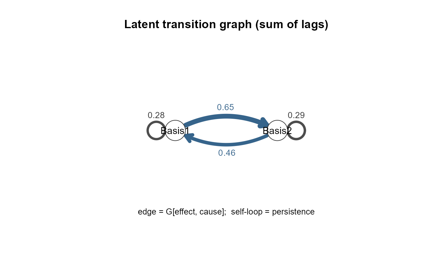
"graph"

The transition graph of \(G_d\): self-loops are persistence, arrows \(q'\to q\) are spillover, widths are proportional to the entries. Unlike a \(y\to b\to y\) bipartite picture this graph is closed, so an asymmetric feedback loop is visible as such.

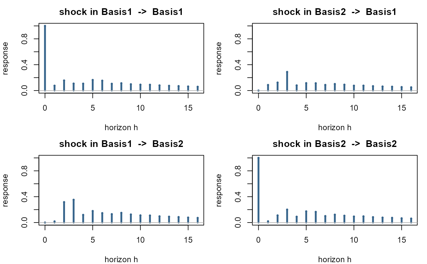
"irf"

Latent impulse responses \(\Psi_h\), a \(Q\times Q\) panel. Since \(G_d\ge 0\) the responses never change sign, so the shape is a decay or a hump and its half-life can be read off.

"lag"

\((G_d)_{qq'}\) as a function of \(d\): how many periods a shock takes to arrive. With \(Q=1\) this is a single bar plot of the lag profile.

"phase"

Phase portrait of \(b_t\mapsto Gb_{t-1}+\theta\) with the fixed point \(\mu_b\) and the eigen-directions. Requires \(D=1\) and \(Q=2\). This is where a monotone relaxation and a true cycle look different; two coefficient series plotted against time do not distinguish them.

See also

nmfkc.ar.latent, nmfkc.ar.latent.inference, plot.nmfkc.ar.stationarity, nmfkc.ar.DOT

Examples

set.seed(1)
Y   <- matrix(abs(rnorm(4 * 60)) + 1, 4, 60)
ar  <- nmfkc.ar(Y, degree = 3)
fit <- nmfkc(ar$Y, ar$A, rank = 2, verbose = FALSE)
lat <- nmfkc.ar.latent(fit)
plot(lat)                  # roots on the unit circle

plot(lat, type = "graph")  # latent transition graph

plot(lat, type = "irf")    # latent impulse responses