Plot method for nmf.gmm objects

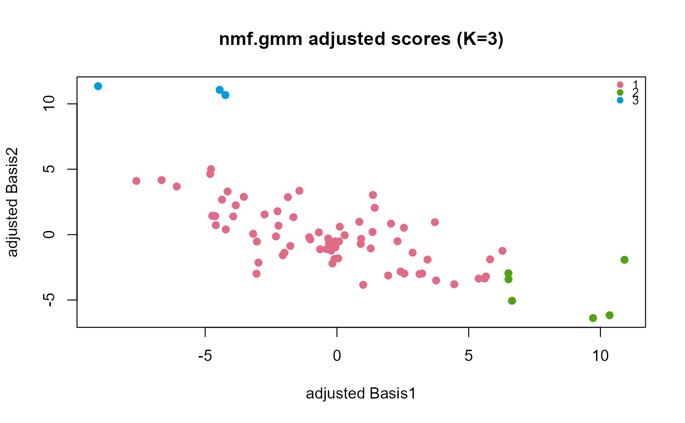
type = "convergence" (default) plots the EM objective ($-\log L$) over iterations. type = "adjusted.scores" draws the cluster scatterplot, coloured by the hard cluster assignment (or by group).

Usage

# S3 method for class 'nmf.gmm'
plot(
  x,
  type = c("convergence", "adjusted.scores", "scores"),
  group = NULL,
  ...
)

Arguments

x: An object of class "nmf.gmm".
type: "convergence" or "adjusted.scores" ("scores" is an alias for the latter).
group: Optional length-N factor/vector to colour the scatterplot by (e.g. known labels). Default NULL colours by x$cluster.
...: Additional graphical parameters passed to plot.

Value

Invisible NULL.

Details

The scatterplot shows the adjusted scores, not the scores. What is drawn is $\bm b_n - C\bm a_n$, the least-squares scores with the covariate effect removed — which is the space the mixture actually acts in, since the model puts the covariate effect in the component means. The distinction matters: on the crabs example the raw scores separate the four true groups no better with a size covariate than without (0.635 versus 0.648, between/within on the first two principal components), while the adjusted space separates them at 4.628. The visible separation is produced by the adjustment, so a panel labelled "scores" would claim something the picture does not show. type = "scores" is accepted as an alias.

The projection depends on the rank: a rank-2 fit is drawn in its own two coordinates (rotating it through prcomp would trade two interpretable part axes for arbitrary ones), a higher rank is projected onto its first two principal components, and a rank-1 fit becomes a strip plot with deterministic stacking.

Development status

Part of the experimental NMF-GMM family: see nmf.gmm. The interface may change in future versions — argument names, defaults and the contents of the returned object are not yet stable.

Examples

# \donttest{
set.seed(1)
Y <- matrix(abs(rnorm(20 * 80)) + 1, 20, 80); A <- rbind(1, rnorm(80))
fit <- nmf.gmm(Y, A, rank = 2, K = 3)
plot(fit, type = "adjusted.scores")

# }