Plot Diagnostics: Original, Fitted, and Residual Matrices as Heatmaps

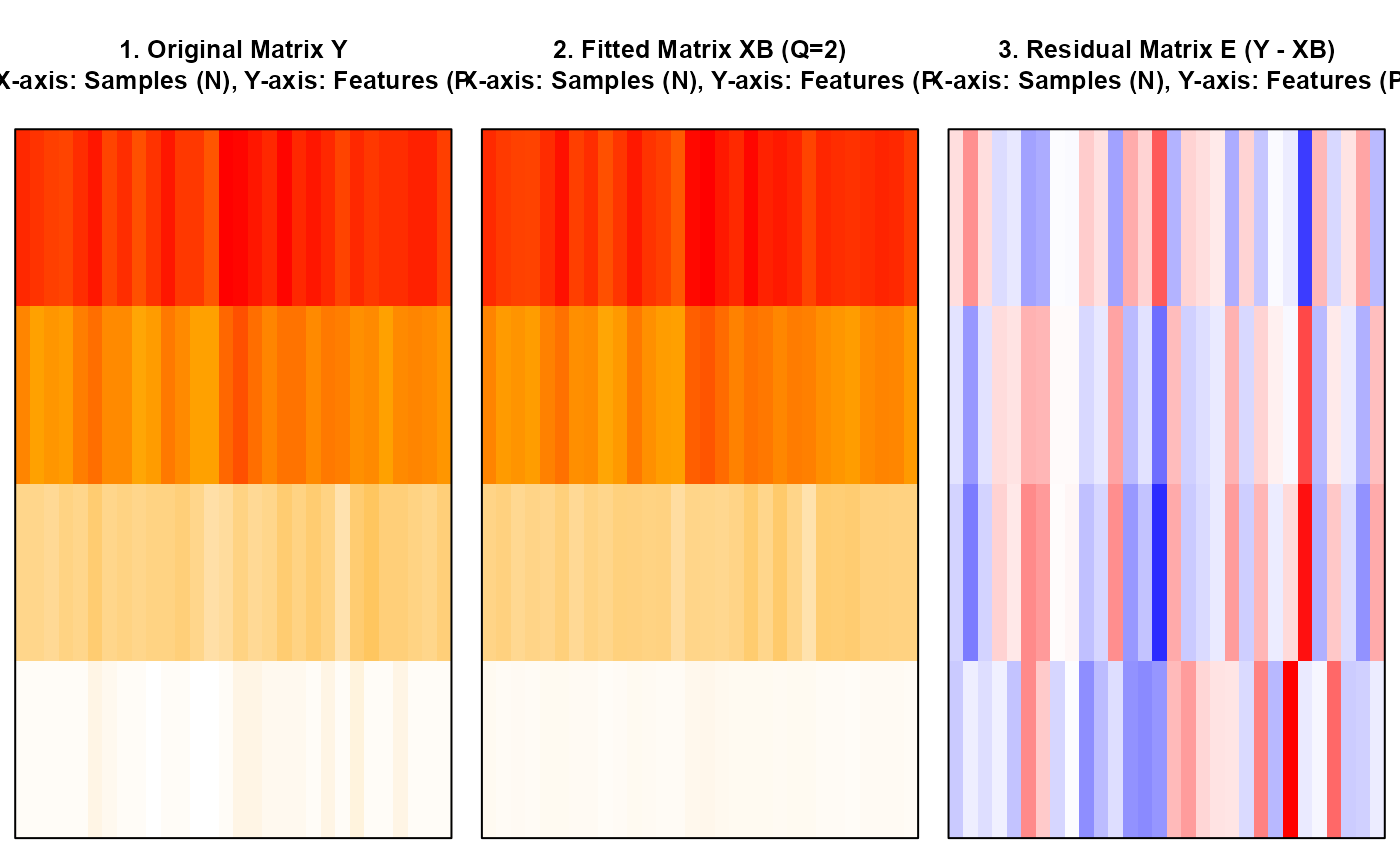
This function generates a side-by-side plot of three heatmaps: the original observation matrix Y, the fitted matrix XB (from NMF), and the residual matrix E (Y - XB). This visualization aids in diagnosing whether the chosen rank Q is adequate by assessing if the residual matrix E appears to be random noise.

The axis labels (X-axis: Samples, Y-axis: Features) are integrated into the main title of each plot to maximize the plot area, reflecting the compact layout settings.

Usage

nmfkc.residual.plot(
  Y,
  result,
  fitted.palette = (grDevices::colorRampPalette(c("white", "orange", "red")))(256),
  residual.palette = (grDevices::colorRampPalette(c("blue", "white", "red")))(256),
  ...
)

Arguments

Y

The original observation matrix (P x N).

result

The result object returned by the nmfkc function.

fitted.palette

A vector of colors for Y and XB heatmaps. Defaults to white-orange-red. For backward compatibility, Y_XB_palette is accepted via ....

residual.palette

A vector of colors for the residuals heatmap. Defaults to blue-white-red. For backward compatibility, E_palette is accepted via ....

...

Additional graphical parameters passed to the internal image calls.

Value

NULL. The function generates a plot.

See also

nmfkc, residuals.nmf

Examples

Y <- t(iris[1:30, 1:4])
result <- nmfkc(Y, rank = 2)
#> Y(4,30)~X(4,2)B(2,30)...
#> 0sec
nmfkc.residual.plot(Y, result)