Quick start: US Presidential Inaugural Addresses

This vignette reproduces the figures used in Section 4 of the companion paper, applied to the US Presidential Inaugural Addresses corpus shipped with the package.

library(ljmds)

1. Load the corpus from CSV

The corpus ships as a CSV in which column 1 is the calendar year and columns 2.. are 0/1 indicators of keyword presence (no source text is included).

d <- ljmds.read.csv("inaugural")
dim(d$X)                  # 59 x 106
#> [1]  59 106
range(d$t)                # 1789 2021
#> [1] 1789 2021
head(d$keywords, 10)
#>  [1] "people"     "government" "nation"     "country"    "power"     
#>  [6] "world"      "citizen"    "time"       "peace"      "man"

2. Joint (h, k) selection

A minimal grid is used here so the vignette builds quickly; a finer grid is recommended in practice (e.g., h.grid = c(8, 10, 15, 20, 25, 30, 40, 50, 70, 100)). The trivial k = 2 split is excluded by leaving 2 out of k.grid (default 3:6).

sel <- ljmds.select(d$X, d$t,
                    h.grid = c(30, 50),
                    k.grid = 3:4)
sel$h.hat
#> [1] 50
sel$k.hat
#> [1] 3
sel$S.hat
#> [1] 0.3310261
round(sel$S, 3)
#>        k3    k4
#> h30 0.261 0.133
#> h50 0.331 0.177

3. Run the pipeline at $(k, h) = (3, 50)$

fit <- ljmds.pipeline(d$X, d$t, h = 50, k = 3)

4. Figures from the paper

Figure 3: cluster centroid trajectories

plot(fit, type = "trajectory")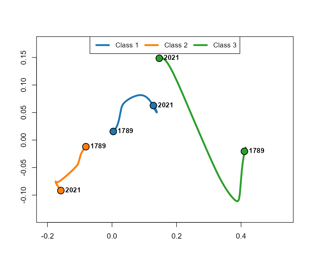

Centroid trajectories on the modified MDS configuration.

Figure 4: Ward dendrogram

plot(fit, type = "dendrogram")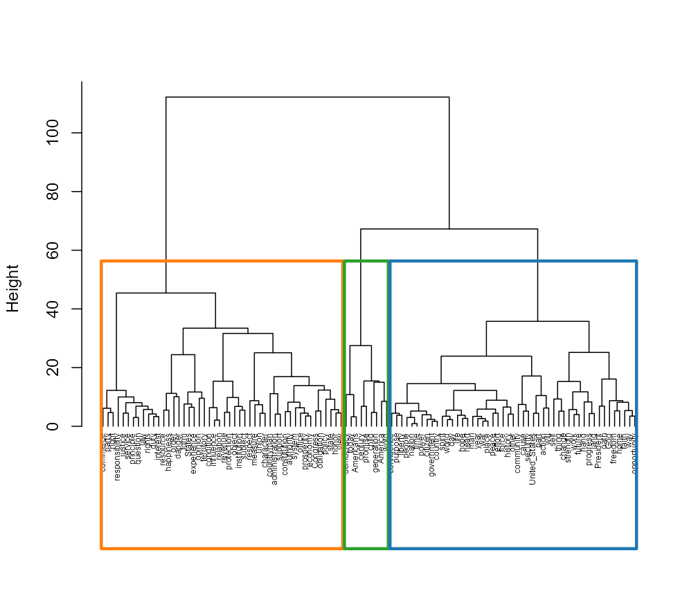

Ward dendrogram on the trajectory distance H.

Figure 5: joint selection heatmap

plot(sel)

Silhouette heatmap S(k, h) with maximizer marker.

Figure 6: time-collapsed MDS map

plot(fit, type = "cmd")

Classical MDS of H, coloured by class.

Figure 7: class mean curves

plot(fit, type = "means")

Class mean occurrence curves.

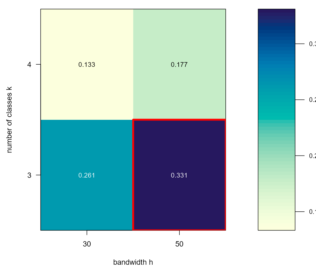
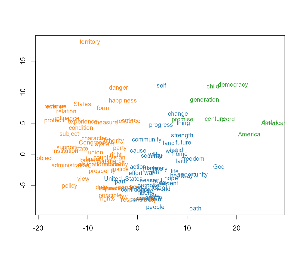
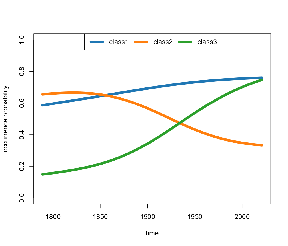
Figure 8: per-class small multiples

plot(fit, type = "panels")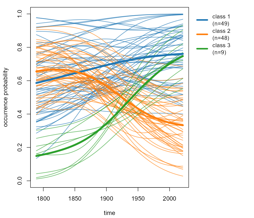

Individual smoothed curves and class means.

Figure 9: animated trajectory map (GIF)

A pre-rendered animation ships with the package; locate it with system.file() and view it directly:

gif_path <- system.file("extdata", "inaugural.gif",
                        package = "ljmds")
gif_path
#> [1] "C:/Users/ksato/AppData/Local/Temp/RtmpOeJTLU/temp_libpath115442fc12dc/ljmds/extdata/inaugural.gif"

browseURL(gif_path)              # open in default browser
# magick::image_read(gif_path)   # or: open in RStudio Viewer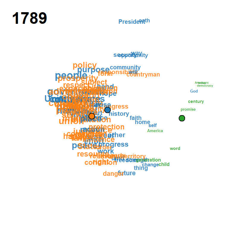

To regenerate the GIF from the fitted object (writes a new file to the current working directory; takes about a minute), uncomment and run:

# gif <- ljmds.animate(fit, file = "inaugural.gif",
#                   trail = 7, fps = 2)