Quick start: Eurovision Song Contest country participation

This vignette reproduces the figures used in Section 6 of the companion paper, applied to the Eurovision Song Contest country participation 1956–2023 (the 2020 contest was cancelled and is absent from the matrix). Unlike the other two examples, there is no text input at all: the rows are contest years, the columns are countries, and the cells are 1 / 0 indicators of whether a given country fielded a contestant in a given year. Source: the MIT-licensed Mirovision dataset of Amsterdam Music Lab.

library(ljmds)

1. Load the corpus from CSV

d <- ljmds.read.csv("eurovision")
dim(d$X)                  # 68 x 52
#> [1] 68 52
range(d$t)                # 1956 2023
#> [1] 1956 2023
head(d$keywords, 10)      # country names
#>  [1] "Andorra"            "Albania"            "Armenia"           
#>  [4] "Austria"            "Australia"          "Azerbaijan"        
#>  [7] "Bosnia_Herzegovina" "Belgium"            "Bulgaria"          
#> [10] "Belarus"

2. Joint (h, k) selection

A minimal grid is used here so the vignette builds quickly; a finer grid is recommended in practice (e.g., h.grid = c(3, 5, 8, 12, 20)). The trivial k = 2 split is excluded by leaving 2 out of k.grid (default 3:6).

sel <- ljmds.select(d$X, d$t,
                    h.grid = c(12, 20),
                    k.grid = 4:5)
sel$h.hat
#> [1] 20
sel$k.hat
#> [1] 5
sel$S.hat
#> [1] 0.4749629
round(sel$S, 3)
#>        k4    k5
#> h12 0.369 0.384
#> h20 0.418 0.475

3. Run the pipeline at $(k, h) = (5, 20)$

fit <- ljmds.pipeline(d$X, d$t, h = 20, k = 5)

4. Figures from the paper

Figure 17: cluster centroid trajectories

plot(fit, type = "trajectory")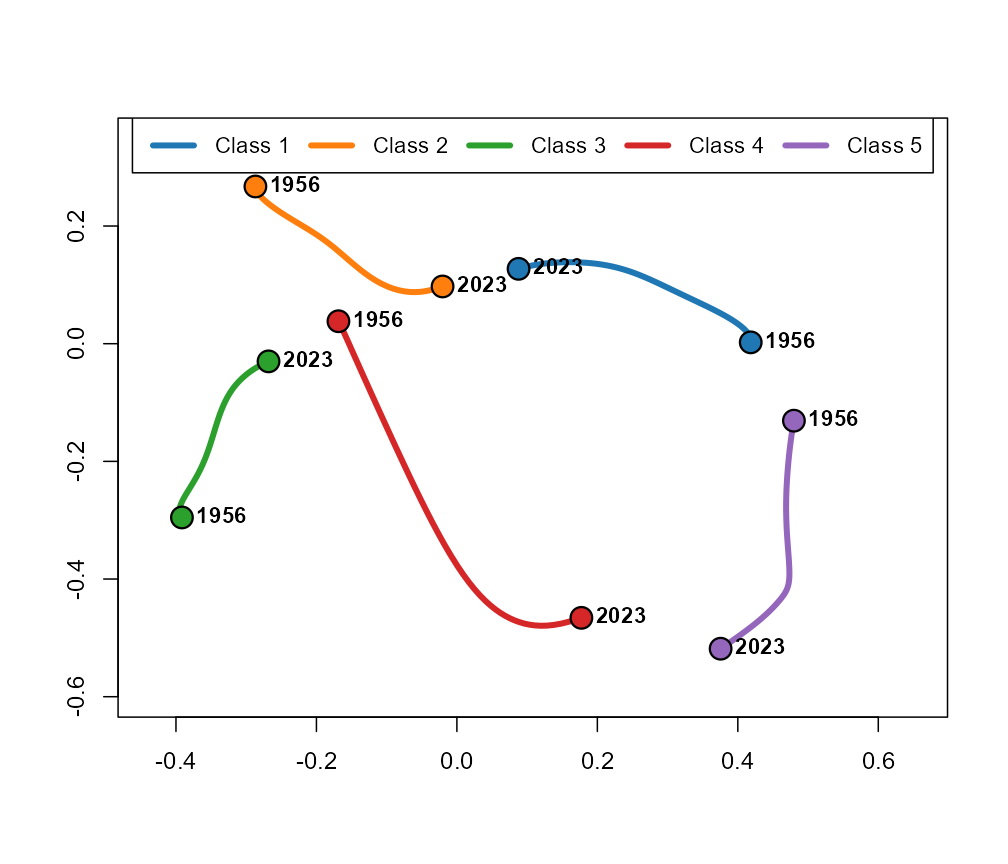

Centroid trajectories on the modified MDS configuration.

Figure 18: class mean participation curves

plot(fit, type = "means")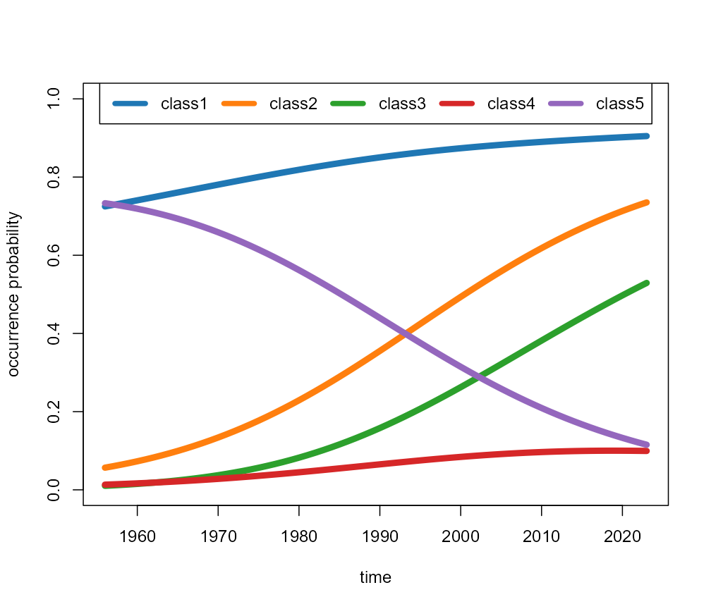

Class mean participation probability curves.

Figure 19: Ward dendrogram

plot(fit, type = "dendrogram")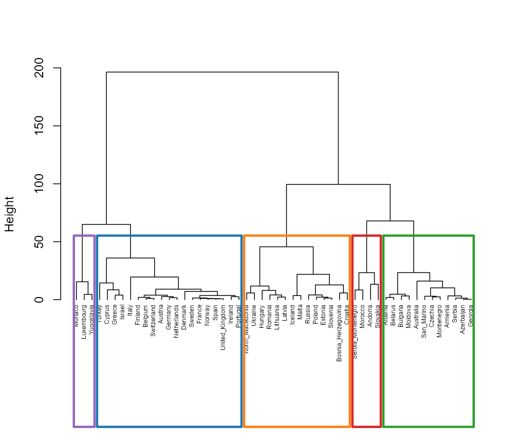

Ward dendrogram on the trajectory distance H.

Figure 20: silhouette selection heatmap

plot(sel)

Silhouette heatmap S(k, h) with maximizer marker.

Figure 21: time-collapsed MDS map

plot(fit, type = "cmd")

Classical MDS of H, coloured by class.

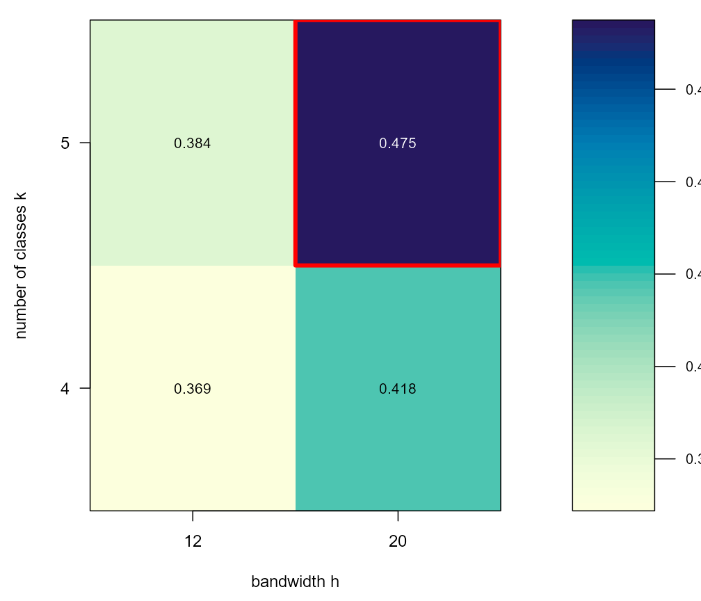
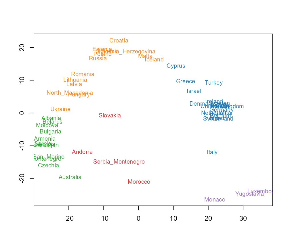
Figure 22: per-class small multiples

plot(fit, type = "panels")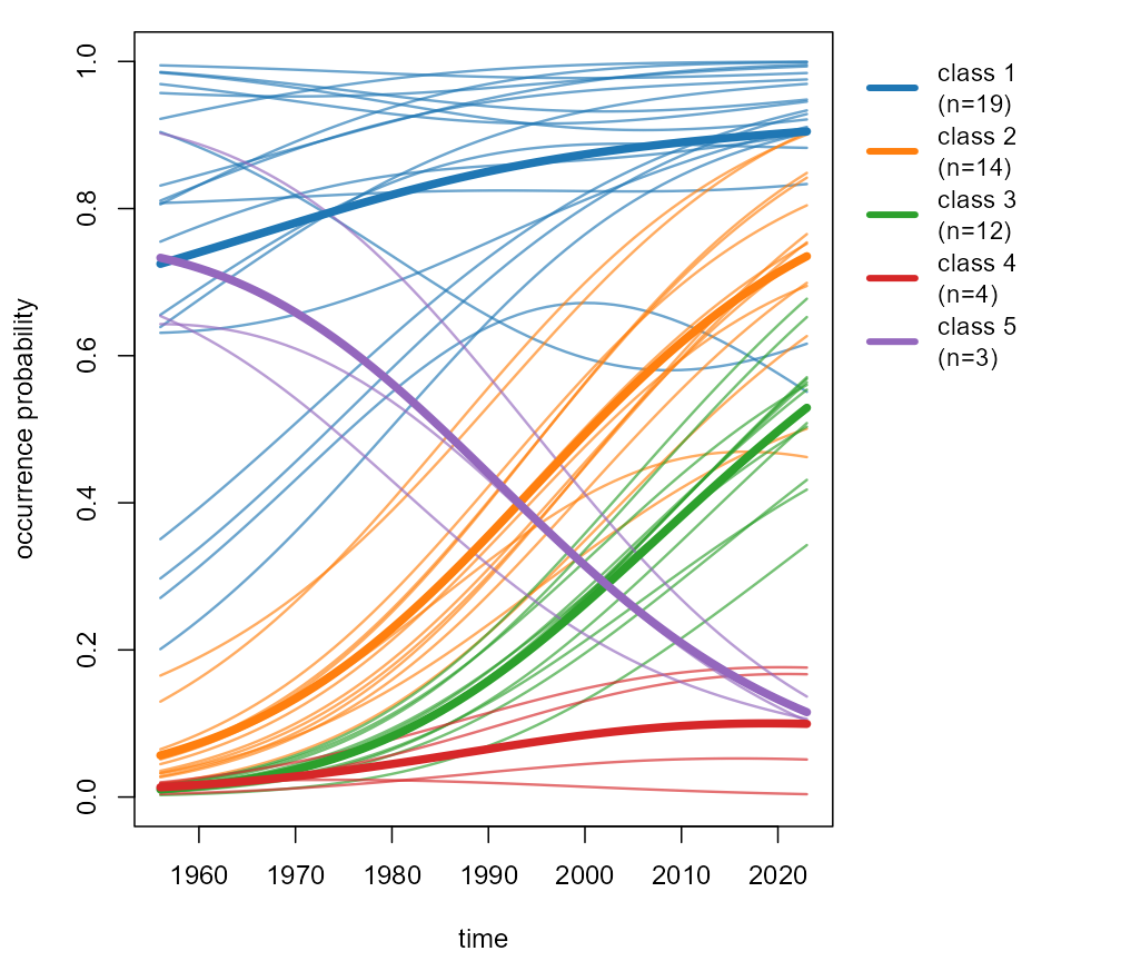

Individual smoothed curves and class means.

Figure 23: animated trajectory map (GIF)

A pre-rendered animation ships with the package; locate it with system.file() and view it directly:

gif_path <- system.file("extdata", "eurovision.gif",
                        package = "ljmds")
gif_path
#> [1] "C:/Users/ksato/AppData/Local/Temp/RtmpOeJTLU/temp_libpath115442fc12dc/ljmds/extdata/eurovision.gif"

browseURL(gif_path)              # open in default browser
# magick::image_read(gif_path)   # or: open in RStudio Viewer

To regenerate the GIF from the fitted object (writes a new file to the current working directory), uncomment and run:

# gif <- ljmds.animate(fit, file = "eurovision.gif",
#                      trail = 7, fps = 2)